Estimating test-retest reliability for Stroop effect
Gang Chen (twitter: @gangchen6)
Preface
Properly estimating test-retest reliability has become a hot topic in recent years. Traditionally, test-retest reliability is conceptualized and quantitatively estimated as intraclass correlation (ICC), whose definition can be found in, for example, this wikipedia page. Even though there is the tricky issue of assessing its uncertainty, the traditional ICC formulation works roughly fine as a point estimate when no or little measurement error is present. However, the adoption of ICC can be problematic when measurement uncertainty becomes an issue in situations where the quantity under study is measured many times with substantial amount of variability. This may be related to the issue of reported low ICC values (“reliability crisis”) in the psychometrics and neuroimaging literature.
A new modeling framework is needed to accurately estimate test-retest reliability with measurement errors properly handled. In experiments where the effect is assessed through many trials, we intend to construct a hierarchical/multilevel model that
1) characterizes/maps the data structure as close to the data structure (or data generative mechanism) as possible, and
2) separates the cross-trial variability from the estimation process of test-retest reliability. It is this hierarchical modeling framework we would like to adopt and demonstrate in this blog. More detailed theoretical discussion from the modeling perspective can be found in the following papers.
-
Haines et al., 2020. Learning from the Reliability Paradox: How Theoretically Informed Generative Models Can Advance the Social, Behavioral, and Brain Sciences (preprint). PsyArXiv.
-
Rouder, J.N., Haaf, J.M., 2019. A psychometrics of individual differences in experimental tasks. Psychon Bull Rev 26, 452–467.
-
Chen et al., 2021. Trial and error: A hierarchical modeling approach to test-retest reliability. NeuroImage 245, 118647.
This blog intends to
a) lay out the structure of a hierarchical modeling framework under which trial-level effects are segregated from the estimation of test-retest reliability;
b) demonstrate the implementation of the hierarchical model using the R package brms with a dataset from a Stroop experiment (Hedge et al., 2018).
Hierarchical modeling framework
Let’s first set the stage for our modeling framework. Suppose that, in a test-retest experiment, the quantity of interest (e.g., reaction time) \(y_{crst}\) is measured at trial \(t\) (\(t=1,2,…,T\)) during each of the two repetitions/sessions (\(r=1,2\)) for subject \(s\) (\(s=1,2,…,S\)) under the condition \(c\) (\(c=1,2\)). The goal is to assess the test-retest reliability for the contrast between the two conditions. Conceptually, the test-retest reliability measures the correlation of the contrast between the two repetitions/sessions. If one adopts the conventional ICC formulation, the data will have to be aggregated by collapsing trial dimension and obtain, for example, the average values \(\overline{y}_{cs\cdot}\). However, test-retest reliability could be underestimated under some circumstances, and the extent of underestimation depends on the relative magnitude of cross-trial variability compared to its cross-subject counterpart (Rouder et al., 2019; Chen et al., 2021). Here we build the following hierarchical model1,
\[\begin{aligned} \text{trial level: }y_{crst} ~ &\sim ~\mathcal D (\alpha_{crs}, \ \sigma_{crs}^2);\\ \text{subject level: }\alpha_{crs}\ &=\ m_{cr}\ +\ \mu_{crs};\\ \text{subject level: }\sigma_{crs}\ &=\ \gamma_{cr}\ +\ \tau_{crs};\\ \text{populatioin level: }\begin{bmatrix} \mu_{11s} \\ \mu_{21s} \\ \mu_{12s} \\ \mu_{22s} \\ \tau_{11s} \\ \tau_{21s} \\ \tau_{12s} \\ \tau_{22s} \end{bmatrix} &\ \sim \ \operatorname{Normal} \left ( \begin{bmatrix} 0 \\ 0 \\ 0 \\ 0 \\ 0 \\ 0 \\ 0 \\ 0 \end{bmatrix},\ \mathbf \Sigma_{8\times 8} \right). \\ \end{aligned}\]Here the distribution \(\mathcal D\) at the trial level can be any probability density that could properly capture the data generative mechanism. The typical distributions for reaction time are Gaussian, Student’s \(t\), exponentially-modified Gaussian, (shifted) log-normal, etc. The two parameters of \(m_{cr}\) and \(\gamma_{cr}\) are the population-level effect and standard deviation under condition \(c\) during repetition \(r\). The variance-covariance matrix \(\mathbf \Sigma_{8\times 8}\) captures the inter-relationships among the subject-level effects \(\mu_{crs}\) and standard deviations \(\tau_{crs}\). We know that, after scaling, the variance-covariance matrix \(\mathbf \Sigma_{8\times 8}\) would show the correlation structure among the four components of \((\mu_{11s},\ \mu_{21s},\ \mu_{12s},\ \mu_{22s})\). Later I will demonstrate how to extract the jewels in the crown from this matrix \(\mathbf \Sigma_{8\times 8}\) and obtain test-retest reliability for various effects. Those parameters (e.g., hyperparameters \(m_{cr}\), \(\mathbf \gamma_{cr}\), \(\mathbf \Sigma_{8\times 8}\)) without a distribution attached will be assigned with some priors in real implementations.
Understanding the modeling formulation is important. Without jotting down a model in mathematical formula, I would have trouble fully grasping a chunk of code (e.g., brms implementation). In fact, usually the model can be directly mapped to the numerical code. I’d like to note the following about the hierarchical model for test-retest reliability -
-
The crucial aspect of the hierarchical model above is that the separation of cross-trial variability – characterized by the variance \(\sigma_{crs}^2\) in the trial-level formulation – from the test-retest reliability (embedded in the variance-covariance matrix \(\boldsymbol \Sigma_{8\times 8}\)) at the subject level. It is this separation that allows the accurate estimation of test-retest reliability through the hierarchical model. It is also because of the lack of this separation in the conventional ICC formulation that leads to the pollution and underestimation of test-retest reliability.
-
The hierarchical model formulated here is parameterized flatly with all the four combinations (indexed by \(c\) and \(r\)). Personally, I consider this parameterization is much more intuitive and more generic. That is, the model considered here is slightly different from all the three papers cited above including my own (Chen et al., 2021).
-
Haines et al. (2020) adopted dummy coding for the two conditions with one condition coded as 1 while the other serves as 0 (reference level). Thus, each slope would correspond to the condition contrast (the effect of interest in the current context) and each intercept is associated with the reference condition per session. A strong assumption was made in Haines et al. (2020) that no correlation exists between the condition contrast and the reference condition as well as for the reference condition between the two repetitions/sessions. In other words, some off-diagonal elements in \(\mathbf \Sigma_{8\times 8}\) were a priori assumed to be 0 in Haines et al. (2020).
-
Rouder et al. (2019) used an indicator variable for the two conditions (0.5 for one condition and -0.5 for the other). Under this coding, each slope is the contrast between the two conditions per session (usually the effect of interest) while each intercept is the average between the two conditions. One underlying assumption with the model in Rouder et al. (2019) was that no correlation exists between a slope (contrast) and an intercept (average). In addition, cross-trial variability was assumed to be constant with no fine structure across conditions/sessions.
-
Chen et al. (2021) utilized the same indicator coding and shared the same underlying assumptions as Rouder et al. (2019).
-
Demo preparation
Here I’ll use a dataset of Stroop task from Hedge et al. (2018) to demonstrate the hierarchical modeling approach to estimating test-retest reliability. The data were collected from 47 subjects who performed Stroop tasks with 2 conditions (congruent, incongruent), 2 sessions (about three weeks apart), 240 trials per condition per session. First, we download the Stroop data from this publicly accessible site and put them in a directory called stroop/. Then, let’s steal some R code (with slight modification) from Haines’s nice blog and rearrange the data a little bit:
library(foreach); library(dplyr); library(tidyr)

data_path <- "stroop/"  # here I assume the download data are stored under directory 'stroop'
files_t1 <- list.files(data_path, pattern = "*1.csv")
files_t2 <- list.files(data_path, pattern = "*2.csv")

# Create a data frame in long format
long_stroop <- foreach(i=seq_along(files_t1), .combine = "rbind") %do% {
  # repetition/session 1
  tmp_t1 <- read.csv(file.path(data_path, files_t1[i]), header = F) %>% mutate(subj_num = i, time = 1)
  # repetition/session 2
  tmp_t2 <- read.csv(file.path(data_path, files_t2[i]), header = F) %>% mutate(subj_num = i, time = 2)
  # Condition (0: congruent, 1: neutral, 2: incongruent), correct (1) or incorrect (0), RT (seconds)
  names(tmp_t1)[1:6] <- names(tmp_t2)[1:6] <- c("Block", "Trial", "Unused", "Condition", "Correct", "RT")
  rbind(tmp_t1, tmp_t2)
}

dat <- long_stroop[long_stroop$Condition!=1,]
Next, to apply the data to our hierarchical model, we flatten the two factors (condition and session) of \(2\times 2\) structure into a dimension of four combinators with the following R code:
dat[dat$Condition==2,'Condition'] <- 'inc' # incongruent
dat[dat$Condition==0,'Condition'] <- 'con' # congruent
dat$com <- paste0(dat$Condition, dat$time) # flatten the two factors
dat$sub <- paste0('s',dat$subj_num).       # subjects
write.table(dat[,c('sub', 'con', 'RT')], file = "stroop.txt", append = FALSE, quote = F, row.names = F)
Now, we have a data table called stroop.txt with the first few lines like this:
sub com RT
s1 con1 0.89078
s1 con1 0.72425
s1 con1 0.49442
s1 inc1 0.80221
s1 inc1 0.8327
...
With 47 subjects, 2 conditions, 2 sessions, and 240 trials per condition per session, there are total 45120 rows in the data table. We purposefully flatten the two factors so that we have a factor with four levels:
levels(dat$com)
These four levels of con1, con2, inc1, and inc2 correspond to congruent during session 1, congruent during session 2, incongruent during session 1, and incongruent during session 2. This coding will allow us to more intuitively/directly parameterize the correlations among all the four combinations. Our goal is to assess the test-retest reliability about the contrast between incongruent and congruent. Keep in mind that the conventional ICC only gave a lackluster reliability estimate of approximately 0.5 (Hedge et al., 2018; Haines et al., 2020; Chen et al., 2021).
OK, now we’re ready for the next adventure.
Estimating test-retest reliability using brms
Let’s implement our hierarchical model with the newly obtained data stroop.txt. Run the following R code:
dat <- read.table('stroop.txt', header=T)
library('brms')
options(mc.cores = parallel::detectCores())
m <- brm(bf(RT ~ 0+com+(0+com|c|sub), sigma ~ 0+com+(0+com|c|sub)), data=dat,
         family=exgaussian, chains=4, iter=1000)
save.image(file = "stroop.RData")
You may be surprised to notice how simple the code is. The only line that codes our model using brm is quite straightforward (if you’re familiar with the specification grammar used by the R package lme4) and it directly maps the data to our hierarchical model. Note that I fit the trial-level effects with an exponentially-modified Gaussian distribution for the probability density \(\mathcal D\) in our hierarchical model above. This implementation may take a few hours (using within-chain parallelization would shorten the runtime), so leave your computer alone and come back later.
Let’s check the results and make sure all the chains behaved properly. The following code
load('stroop.RData')
summary(m)
reveals the summarized results:
Group-Level Effects:
~sub (Number of levels: 47)
                                 Estimate Est.Error l-95% CI u-95% CI  Rhat Bulk_ESS Tail_ESS
sd(comcon1)                         0.052     0.005    0.043    0.064 1.009      216      190
sd(comcon2)                         0.058     0.006    0.048    0.070 1.007      256      297
sd(cominc1)                         0.072     0.007    0.060    0.088 1.009      244      521
sd(cominc2)                         0.061     0.005    0.051    0.073 1.003      369      566
sd(sigma_comcon1)                   0.377     0.037    0.312    0.459 1.004      521      823
sd(sigma_comcon2)                   0.436     0.040    0.366    0.524 1.004      593      766
sd(sigma_cominc1)                   0.381     0.038    0.311    0.466 1.002      524      662
sd(sigma_cominc2)                   0.412     0.041    0.343    0.502 1.001      655     1067
cor(comcon1,comcon2)                0.668     0.079    0.499    0.806 1.008      284      484
cor(comcon1,cominc1)                0.884     0.038    0.798    0.943 1.007      579     1103
cor(comcon2,cominc1)                0.480     0.106    0.256    0.674 1.003      453      874
cor(comcon1,cominc2)                0.651     0.082    0.474    0.796 1.006      339      535
cor(comcon2,cominc2)                0.901     0.034    0.823    0.952 1.002      844     1261
cor(cominc1,cominc2)                0.607     0.088    0.416    0.761 1.003      492      739
cor(comcon1,sigma_comcon1)          0.646     0.087    0.449    0.795 1.002      541      810
cor(comcon2,sigma_comcon1)          0.563     0.095    0.351    0.725 1.003      643     1024
cor(cominc1,sigma_comcon1)          0.660     0.087    0.472    0.812 1.006      549      967
cor(cominc2,sigma_comcon1)          0.601     0.093    0.398    0.762 1.002      637     1282
cor(comcon1,sigma_comcon2)          0.467     0.107    0.245    0.659 1.002      448      727
cor(comcon2,sigma_comcon2)          0.652     0.080    0.472    0.792 1.002      660      822
cor(cominc1,sigma_comcon2)          0.455     0.108    0.225    0.644 1.002      543     1089
cor(cominc2,sigma_comcon2)          0.767     0.065    0.624    0.870 1.003      891     1028
cor(sigma_comcon1,sigma_comcon2)    0.743     0.075    0.566    0.864 1.000      977     1598
cor(comcon1,sigma_cominc1)          0.521     0.105    0.301    0.700 1.006      548      916
cor(comcon2,sigma_cominc1)          0.330     0.118    0.081    0.547 1.002      621      773
cor(cominc1,sigma_cominc1)          0.716     0.071    0.548    0.836 1.001      797     1066
cor(cominc2,sigma_cominc1)          0.505     0.100    0.288    0.683 1.000      686      875
cor(sigma_comcon1,sigma_cominc1)    0.867     0.051    0.741    0.946 1.002     1014     1615
cor(sigma_comcon2,sigma_cominc1)    0.627     0.096    0.417    0.786 1.002      852     1106
cor(comcon1,sigma_cominc2)          0.333     0.118    0.090    0.549 1.004      494      749
cor(comcon2,sigma_cominc2)          0.428     0.113    0.179    0.630 1.000      617      993
cor(cominc1,sigma_cominc2)          0.427     0.109    0.186    0.618 1.001      574      962
cor(cominc2,sigma_cominc2)          0.669     0.078    0.494    0.797 1.001      719     1046
cor(sigma_comcon1,sigma_cominc2)    0.638     0.092    0.441    0.796 1.000      988     1408
cor(sigma_comcon2,sigma_cominc2)    0.912     0.037    0.821    0.964 1.001     1201     1537
cor(sigma_cominc1,sigma_cominc2)    0.659     0.090    0.457    0.808 1.001     1060     1283

Population-Level Effects:
              Estimate Est.Error l-95% CI u-95% CI  Rhat Bulk_ESS Tail_ESS
comcon1          0.641     0.008    0.625    0.658 1.020      113      134
comcon2          0.620     0.009    0.603    0.636 1.023      145      337
cominc1          0.705     0.012    0.683    0.730 1.014      126      119
cominc2          0.663     0.010    0.644    0.682 1.019      144      306
sigma_comcon1   -2.732     0.062   -2.855   -2.606 1.012      173      359
sigma_comcon2   -2.805     0.069   -2.945   -2.670 1.015      192      346
sigma_cominc1   -2.249     0.061   -2.367   -2.121 1.007      203      429
sigma_cominc2   -2.438     0.065   -2.562   -2.308 1.013      267      436

Family Specific Parameters:
     Estimate Est.Error l-95% CI u-95% CI  Rhat Bulk_ESS Tail_ESS
beta    0.186     0.001    0.184    0.189 1.003     4082     1369
In the summary above, there is a lot of information to unpack at various levels (population, condition, correlation, standard deviation, etc). For example, you may find the 28 estimated correlations for the big matrix \(\mathbf \Sigma_{8\times 8}\), which is our current focus – those estimated values do seem to justify our adoption of a complex structure for \(\mathbf \Sigma_{8\times 8}\). But first, we should be happy that the four chains were well-behaved (\(\hat R < 1.05\)). In addition, we can use posterior predictive checks to verify the model quality:
pp_check(m, ndraws = 100)
which shows that our model did a pretty good job - the simulated data (green cloud) based on the model fit well with the original RT data (black density curve):
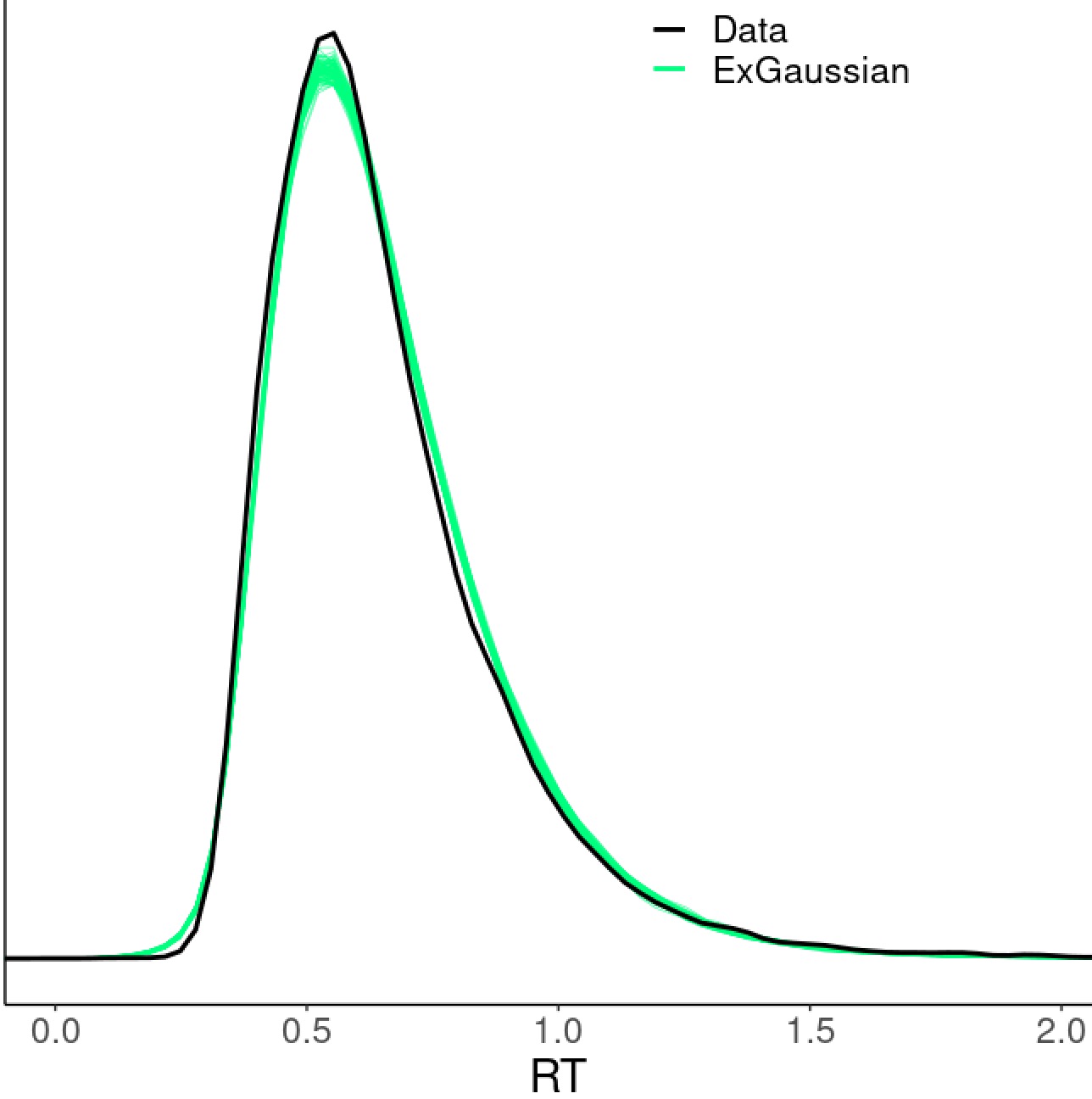
Is there any room for model improvement? Remember that we used exponentially-modified Gaussian to fit the data (distribution \(\mathcal D\) in the model) at the trial level. One may try other distributions such as shifted log-normal (as preferred in Haines et al. (2020)), Gaussian, inverse Gaussian, or Student’s \(t\). In the current case, those alternative distributions could not compete with the exponentially-modified Gaussian as visually illustrated through posterior predictive checks as Fig. 5 in Chen et al. (2021). Comparisons among these models can also be quantitively assessed through leave-one-out cross-validation using the function loo in brms. Keep in mind that even though exponentially-modified Gaussian worked well for this particular dataset, a different distribution (e.g., shifted log-normal) might be more appropriate for another dataset.
It’s time to estimate the test-retest reliability! How to extract it from the model output? All the information is embedded in the variance-covariance matrix \(\mathbf \Sigma_{8\times 8}\). Here comes our finale2:
S   <- VarCorr(m, summary=F)                                   # retrieve draws for the Sigma matrix
C   <- matrix(c(1,0,-1,0,0,1,0,-1), ncol=2, nrow=4)            # matrix for the contrast between the 2 conditions
vc  <- apply(S$sub$cov[,1:4,1:4], 1, function(x) t(C)%*%x%*%C) # compute the var-cov matrix across the 2 sessions for the contrast
trr <- vc[2]/sqrt(vc[1]*vc[4])                                 # assemble draws for TRR
plot(density(trr), xlab='Test-Retest Reliability')             # plot TRR distribution
dens <- density(trr)
dens$x[which.max(dens$y)]                                      # show the peak of the TRR density curve
The plot below shows the posterior distribution of test-retest reliability for cognitive inhibition effect (reaction time difference between incongruent and congruent conditions). Based on our hierarchical model, the mode (peak) for the test-retest reliability of the Stroop dataset is about 0.72, indicating that the underestimation by the conventional ICC(3,1) \(\simeq \) 0.5 is quite substantial. The “reliability crisis” in psychometrics and neuroimaging might be partly caused by improper modeling. The reason for this large extent of underestimation is due to the substantial amount of cross-trial variability compared to cross-subject variability. See more explanation in Chen et al. (2021) regarding the intriguing issue of cross-trial variability as well as the crucial role of trial sample size relative to the subject sample size.
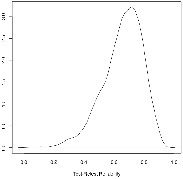
Both Chen et al. (2021) and Haines et al., (2020) used this Stroop dataset as a demo. It is worth noting that the estimated test-retest reliability here is similar to Chen et al. (2021) but to some extent different from Haines et al. (2020). The different results in Haines et al. (2020) were likely due to the stronger assumptions by Haines et al. (2020) regarding the variance-covariance structure in \(\mathbf \Sigma_{8\times 8}\). In fact, the summary(m) output above from brms seems to indicate the violation of their strong assumptions.
-
Thanks to Donald Williams for suggesting the incorporation of correlations between location and scale parameters in this twitter thread ↩
-
Thanks to Michael Freund for suggesting an improvement upon my previous approach to assembling the posterior distribution. ↩